Notes on Imprecise Probability (I): The Ternary Probability Simplex and Credal Sets [imprecise-probability-ternary-simplex-and-credal-sets]

2026-08-31
note
Imprecise probability
A geometric introduction to ternary probability simplices, linear-vacuous models, gambles, and expectation constraints

At the end of last month, I attended the biennial Summer School on Imprecise Probabilities in Munich, Germany. Overall, I found the course very interesting. I did feel, however, that some concepts were not emphasized or explained as thoroughly as they could have been. A great many details were introduced all at once, and in quite a few places I simply could not make sense of an idea after hearing it only once.

I have therefore decided to work through what I learned and reorganize it in a way that suits me better. Starting from the existing slides, I will try to explain the points that interested or confused me in a more intuitive way. These notes will give me something to revisit later and may also offer beginners a useful route into the subject. Today is the last day of August; from now on, I will try to publish at least one note every month. This should become a series of four or five posts, which I hope to finish by the end of the year :)

The course materials are available here. Videos from the previous summer school can also be found on YouTube here.

A geometric interpretation of the ternary probability simplex

Early in the course, the ternary probability simplex was introduced geometrically. This triangle appears constantly in papers about credal sets, usually accompanied by an appeal to some kind of “geometric intuition.”

I do not think that many written explanations make the simplex sufficiently transparent. When I first encountered the idea, for example, I could see the triangle but could not immediately understand where it had come from, let alone quickly plot a probability distribution inside it. Here is my attempt to explain it from the beginning.

Why does a ternary probability distribution become a triangle?

First, why is the ternary probability simplex a triangle?

At first glance the association seems almost self-evident: three outcomes, therefore a triangle. It is then tempting to assume that four outcomes should give a quadrilateral and five outcomes a pentagon. But that is not what happens.

Suppose the sample space contains only three elementary outcomes:

\Omega=\{\omega_1,\omega_2,\omega_3\}.

A probability distribution can be represented by a vector $p=(p_1,p_2,p_3)$ , where $p_i=P(\omega_i)$ .

Probabilities must first satisfy the normalization condition

p_1+p_2+p_3=1.

If we regard $p_1,p_2,p_3$ as coordinates in three-dimensional space, this equation describes a plane.

So normalization alone does not initially give us a triangle; it gives us a plane. Clearly, however, not every point on that plane is a valid probability distribution. Probabilities must also be nonnegative:

p_1\geq 0,\qquad p_2\geq 0,\qquad p_3\geq 0.

These three inequalities restrict us to the first octant. The intersection of that octant with the normalization plane

p_1+p_2+p_3=1

is exactly a triangle. Its three vertices are

(1,0,0),\qquad(0,1,0),\qquad(0,0,1),

corresponding to distributions that place all their probability mass on $\omega_1$ , $\omega_2$ , and $\omega_3$ , respectively.

Here is an illustration:

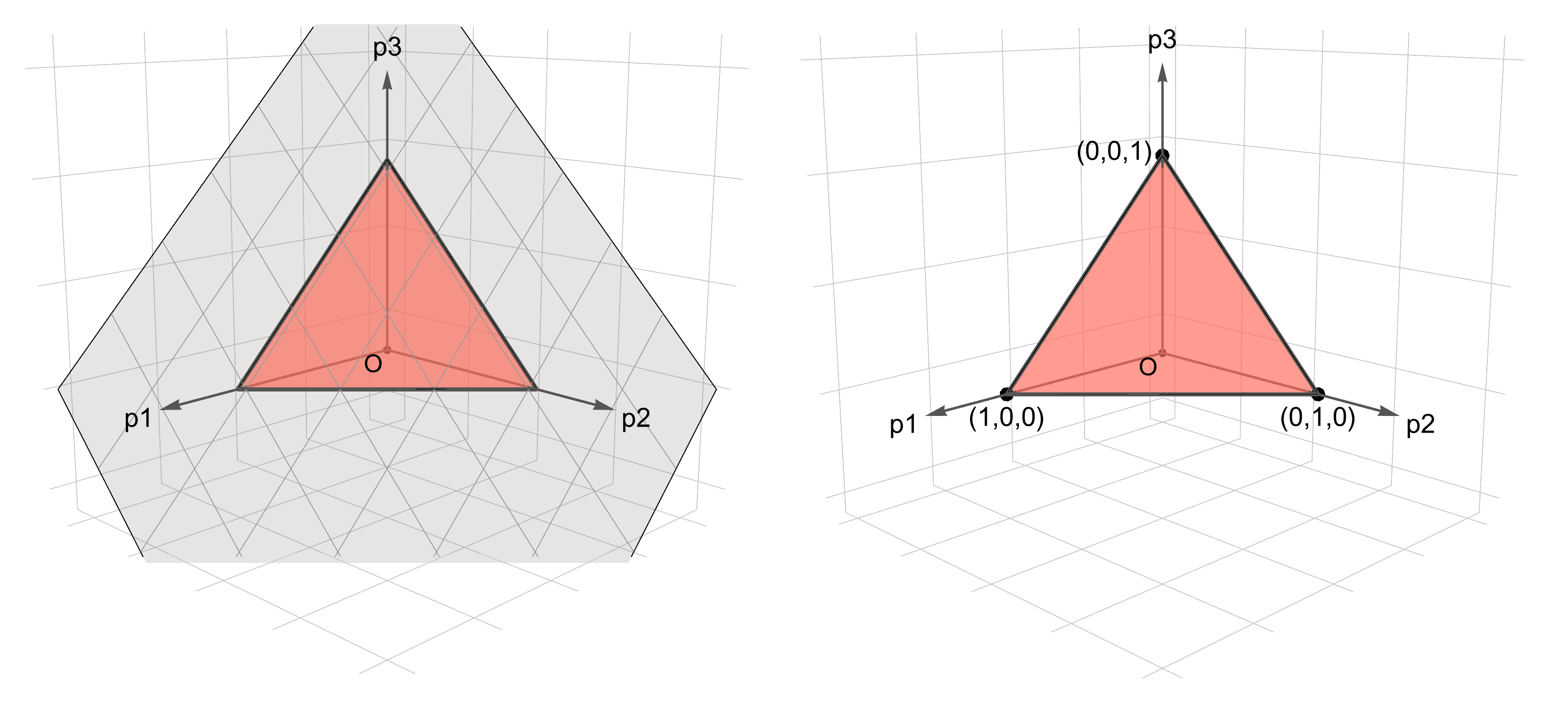
The panel on the left shows the construction I have in mind. The gray region is the entire normalization plane, which extends infinitely in every direction. The red part is all that remains after imposing nonnegativity. Viewed from the right angle, the red triangle faces us directly and becomes the familiar two-dimensional diagram. The triangle is therefore not an arbitrary drawing motivated by the fact that there are three events; it is the geometric result of normalization and nonnegativity acting together.

The same reasoning extends immediately. With $n$ elementary outcomes, the probability vector satisfies

p_1+\cdots+p_n=1,\qquad p_i\geq 0.

The result is an $(n-1)$ -dimensional simplex. A distribution over four outcomes corresponds to a three-dimensional tetrahedron, not a quadrilateral in the plane. Five outcomes give a four-dimensional simplex, which can no longer be drawn in full in ordinary three-dimensional space.

This also explains why papers on imprecise probability so often use ternary examples: three outcomes are the only case that is both nontrivial and easy to draw on paper. The binary simplex is merely a line segment, and a credal set is just an interval on that segment—not much to look at. From four outcomes onward, the picture becomes three-dimensional and harder to reason about visually.

How should we read coordinates inside the triangle?

The course slides say that the coordinate associated with a vertex should be measured from the edge opposite that vertex. The rule is convenient and easy to apply, but when I first read it, it felt rather abrupt: I could see that this was how the diagram worked, but not why.

From the construction above, the answer becomes clearer. Each probability is simply the corresponding coordinate in three-dimensional space. When the normalization plane is represented as a flat triangle, that coordinate turns into a distance. Similar triangles show that the ratio of distances is exactly the ratio of probabilities.

More concretely, fix $p_1=c$ . The remaining constraints are

p_2+p_3=1-c,\qquad p_2,p_3\geq 0.

Within the normalization plane, these conditions describe a line segment. When $c=0$ , the segment is the edge opposite $\omega_1$ , namely the edge on which $p_1=0$ . When $c=1$ , it collapses to the vertex $\omega_1$ . Intermediate values of $c$ interpolate proportionally between these two cases: the segment has $(1-c)$ times the length of the opposite edge, and it lies a fraction $c$ of the way from that edge toward the vertex. Thus $p_1$ is represented by the distance from the point to the edge opposite $\omega_1$ , normalized by the height of the whole triangle.

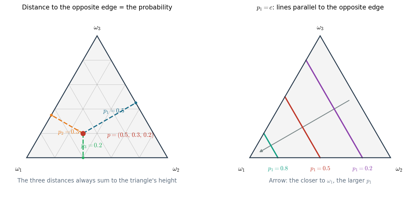
The left panel shows a point $p=(0.5,0.3,0.2)$ . Draw a perpendicular from the point to each edge. After normalizing those three distances by the height of the triangle, they are exactly $0.5$ , $0.3$ , and $0.2$ . Their sum is constant—equal to the triangle's height—a fact known in geometry as Viviani's theorem (or so AI tells me). Here it is simply the condition $p_1+p_2+p_3=1$ in different clothing. In three-dimensional coordinates, normalization is a plane equation; inside the triangle, it says that the three perpendicular distances have a constant sum. To me, this is the real meaning of the rule stated in the slides.

The right panel gives another way to read the same geometry. The equation $p_1=c$ describes a family of lines parallel to the edge opposite $\omega_1$ , and $p_1$ grows as the line moves toward the vertex $\omega_1$ . In practice, there is no need to measure perpendicular distances. To plot $(0.5,0.3,0.2)$ , simply intersect the line $p_1=0.5$ with the line $p_2=0.3$ ; $p_3$ will automatically be correct, because only two of the three constraints are independent.

The linear-vacuous model in the ternary probability simplex

Next consider the linear-vacuous model in the ternary probability simplex. The course sometimes described this as a kind of neighborhood, but more precisely it is a linear-vacuous mixture, also commonly called an $\varepsilon$ -contamination model.

The slides show that its credal set is a triangle. That immediately raised a question for me: why does the credal set remain triangular? I did not find a written explanation, but after thinking about it, I believe the answer is simply vector arithmetic.

Start with a reference probability distribution

p^0=(p^0_1,p^0_2,p^0_3),

and allow a proportion $\varepsilon$ of the probability mass to come from a completely unknown distribution $q$ . A resulting distribution then takes the form

p=(1-\varepsilon)p^0+\varepsilon q,\qquad q\in\Delta_2,

where $\Delta_2$ is the full ternary probability simplex.

The corresponding credal set is therefore

K_\varepsilon =\left\{(1-\varepsilon)p^0+\varepsilon q:q\in\Delta_2\right\}.

Geometrically, this is an operation on the vector $p^0$ .

Represent $p^0$ by the directed segment from the origin to the point $p^0=(p^0_1,p^0_2,p^0_3)$ . Multiplication by $(1-\varepsilon)$ scales that vector: it still points in the same direction but becomes shorter, with an $\varepsilon$ fraction removed by the “contamination.” Notice that the components of $(1-\varepsilon)p^0$ now sum to only $1-\varepsilon$ . The vector no longer lies in the normalization plane; it is short of $\varepsilon$ units of probability mass. The term $\varepsilon q$ restores the missing mass. Since $q$ may be any point in the simplex, $\varepsilon q$ is the whole triangle $\Delta_2$ scaled down by a factor of $\varepsilon$ .

Adding a fixed vector to a small triangle gives the same small triangle translated to a new position. This is why the linear-vacuous credal set remains a triangle: it is the image of $\Delta_2$ under an affine transformation—first a scaling by $\varepsilon$ , then a translation by $(1-\varepsilon)p^0$ . Affine transformations map triangles to triangles without adding any edges.

There is another form of the equation that is even easier to see in the diagram:

p-p^0=\varepsilon(q-p^0).

Starting from $p^0$ , we may move in any direction, but only by an $\varepsilon$ fraction of the distance we could originally travel. In other words, the entire simplex $\Delta_2$ undergoes a homothety centered at $p^0$ with scale factor $\varepsilon$ . When $\varepsilon=0$ , the set collapses to a single point, giving a precise probability distribution. When $\varepsilon=1$ , it fills the entire simplex, representing complete ignorance—the vacuous model.

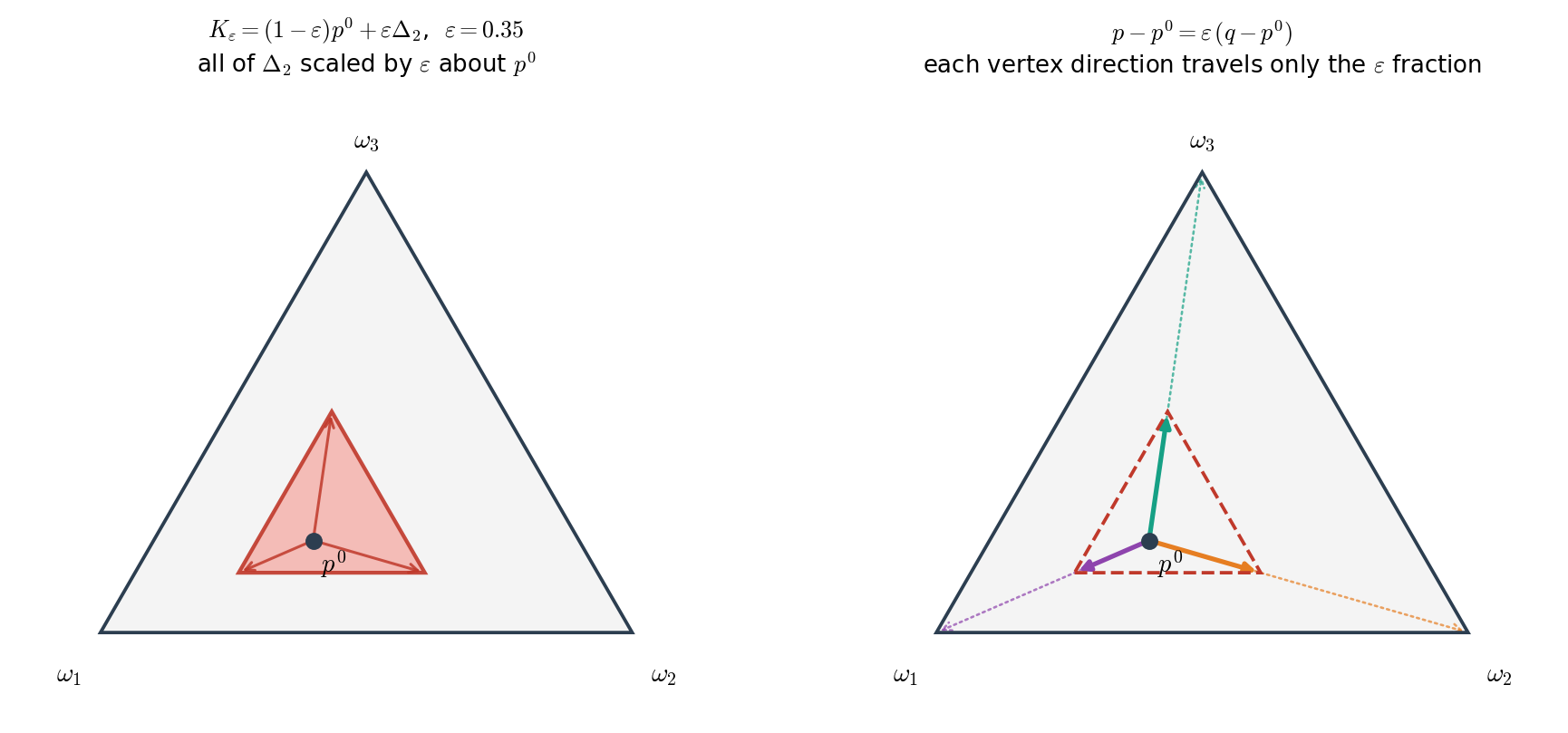
The left panel shows the result, while the right panel shows the construction. The three thick arrows point from $p^0$ toward the three vertices; the dotted extensions indicate where they would end without the scaling. The three edges of the small triangle are parallel to their counterparts in the large one, and corresponding vertices point in the same directions—the signature of a homothety. This also answers a question I initially had: why is the “center” of the small triangle not in the middle of the large one? Because its center is $p^0$ , not the uniform distribution. Wherever $p^0$ is displaced, the whole small triangle is displaced with it.

The gambling interpretation of imprecise probability

While learning imprecise probability theory, I noticed that gambling is used constantly to explain probability. This makes historical sense, since probability theory itself has deep roots in games of chance. The kind of gambling meant here, however, is rather different from the mahjong or card games I had previously associated with the word.

In this interpretation, the bet concerns whether some event $A$ occurs.

Define a ticket by

I_A(\omega)= \begin{cases} 1,&\omega\in A,\\ 0,&\omega\notin A. \end{cases}

If $A$ occurs, the ticket pays one unit of money; otherwise it pays nothing. The particular monetary unit does not matter. Its only purpose is to normalize the payoff to either $0$ or $1$ .

Suppose you buy the ticket for a price $p$ . Your net payoff is

I_A-p.

If the event occurs, you receive $1-p$ ; if it does not, you receive $-p$ .

We can also view the same transaction from the seller's side. You sell the contract for $p$ , receiving $p$ now, but later must pay out according to $I_A$ : one unit if $A$ occurs and zero otherwise. The seller's net payoff is

p-I_A.

Here “selling” means taking the seller's side of this gambling contract, not merely reselling a lottery ticket that you received for free.

Considering both the buying and selling sides gives a behavioral interpretation of probability.

There is a crucial idealization hidden here. If $p$ is called your “fair price” for $A$ , then around that price you must be willing to take either side of the transaction. In other words, your opponent is allowed to choose which direction to bet against you. Dutch-book arguments for precise subjective probability operate under exactly this assumption.

Thus $p$ is not merely your informal guess at what the ticket might be worth. It is a betting quotient that constrains the choices you are prepared to make. If your quoted prices are mutually inconsistent, an opponent may be able to combine several transactions—each acceptable on its own—into a portfolio that makes you lose regardless of the outcome.

Where do nonnegativity, normalization, and additivity come from?

Nonnegativity is straightforward. The ticket $I_A$ never pays less than zero, so receiving it for free can never hurt you. If you assign it a negative price $p<0$ , you are effectively willing to pay someone to take it from you: the opponent receives both $I_A$ and the additional amount $|p|$ . Their net payoff is at least $I_A+|p|\geq|p|>0$ in every state. That is an immediate Dutch book. A coherent price therefore cannot be negative.

Nor should the price of an event ticket exceed $1$ , because the largest possible payoff of $I_A$ is $1$ . If you buy it for $p>1$ , your best possible net payoff is $1-p<0$ and your worst is $-p$ . You lose in every case. Hence

0\leq P(A)\leq 1.

Normalization is equally simple. The ticket associated with the certain event $\Omega$ always pays $1$ , so its fair price must be

P(\Omega)=1.

If its price were below $1$ , an opponent could buy it and lock in a profit of $1-P(\Omega)>0$ . If its price were above $1$ , buying it would guarantee a loss. The two sides leave only the price $1$ . By the same reasoning, the ticket for the impossible event always pays zero and must have price zero.

For additivity, suppose that $A$ and $B$ are disjoint. Then

I_{A\cup B}=I_A+I_B.

Buying one ticket that pays $1$ when either $A$ or $B$ occurs produces exactly the same payoff in every state as buying one $A$ ticket and one $B$ ticket separately.

Two portfolios with identical state-by-state payoffs should have the same price. Otherwise, one could buy the cheaper portfolio and sell the more expensive one for a risk-free profit. Therefore

P(A\cup B)=P(A)+P(B),\qquad A\cap B=\varnothing.

From this perspective, the axioms of probability are not simply postulated; they follow from the requirement that a system of prices contain no obvious arbitrage.

Whether this is genuinely more intuitive than accepting the probability axioms directly is a matter of taste. To me, it feels more like a behavioral wrapper around those axioms than the one uniquely correct philosophy of probability. The one place where I do find it useful is that it tells us exactly where the theory can be relaxed. Classical theory requires the buying and selling prices to coincide; imprecise probability drops this requirement and allows the buying price to be strictly lower than the selling price. The gap between them represents your ignorance. Viewed this way, a credal set is not an arbitrary extra set attached to probability theory: it is the geometry of a bid–ask spread.

Constraining a credal set with expectations

To be honest, I understood almost none of this part during the course. This may be one reason why imprecise probability remains a niche subject: the entry barrier feels higher than in machine learning. The concepts, notation, and gambling interpretation were all piled on at once, and I genuinely could not follow them. I will therefore rebuild this part from the ground up, at least far enough to make it fit my intuition. I will not try to cover every detail.

What are the limitations of lower and upper probabilities alone?

The lower and upper probabilities introduced earlier are easy to understand. For example,

\underline P(\{\omega_1\}) \leq p_1 \leq \overline P(\{\omega_1\}).

In the ternary probability simplex, $p_1=c$ is a line parallel to one edge of the triangle. Likewise, $p_2=c$ and $p_3=c$ are parallel to the other two edges. Some statistical methods can produce constraints of this form.

In a three-outcome space, every event has one of only a few basic forms: a single outcome, a union of two outcomes, the full space, or the empty set. Since

p_1+p_2=1-p_3,

constraining the probability of a union of two outcomes is still, in essence, just constraining the remaining coordinate.

Consequently, if we cut the ternary simplex using only lower and upper probabilities of events, the resulting edges are all parallel to edges of the original triangle. The shapes are regular, but their expressive power is limited. There are only three directions and at most six edges, so in the linear case a hexagon is the most complicated shape we can obtain. All the shapes in the earlier model-comparison figure fall within this limit. But what if we want a convex credal set with slanted or less regular edges? Such a set is difficult to describe using only these constraints.

From event indicators to general gambles

The natural next step is to stop restricting ourselves to event indicators with coefficients only $0$ or $1$ , and instead allow arbitrary payoff functions.

Represent a gamble by

f=(f_1,f_2,f_3),

where $f_i$ is the payoff when outcome $\omega_i$ occurs. When I first encountered this object, I had no idea what it was supposed to mean. I now realize that it is simply a discrete function assigning a value to each possible outcome.

Under a probability distribution $p=(p_1,p_2,p_3)$ , its expectation is

E_p[f] =f_1p_1+f_2p_2+f_3p_3 =p\cdot f.

This is just an expression of the form

ap_1+bp_2+cp_3.

The coefficients $a,b,c$ are no longer mysterious constants: they are the payoffs of the gamble in the three possible outcomes. By changing them, we obtain lines with different slopes in the simplex.

We can therefore impose lower and upper bounds on the expectation:

\underline E(f) \leq f_1p_1+f_2p_2+f_3p_3 \leq \overline E(f).

Geometrically, the equation

f_1p_1+f_2p_2+f_3p_3=c

describes a line within the normalization plane, while an inequality describes the half-plane on one side of that line.

Because $f_1,f_2,f_3$ may be arbitrary, the line need not be parallel to an edge of the triangle. It can cut the probability simplex at any angle.

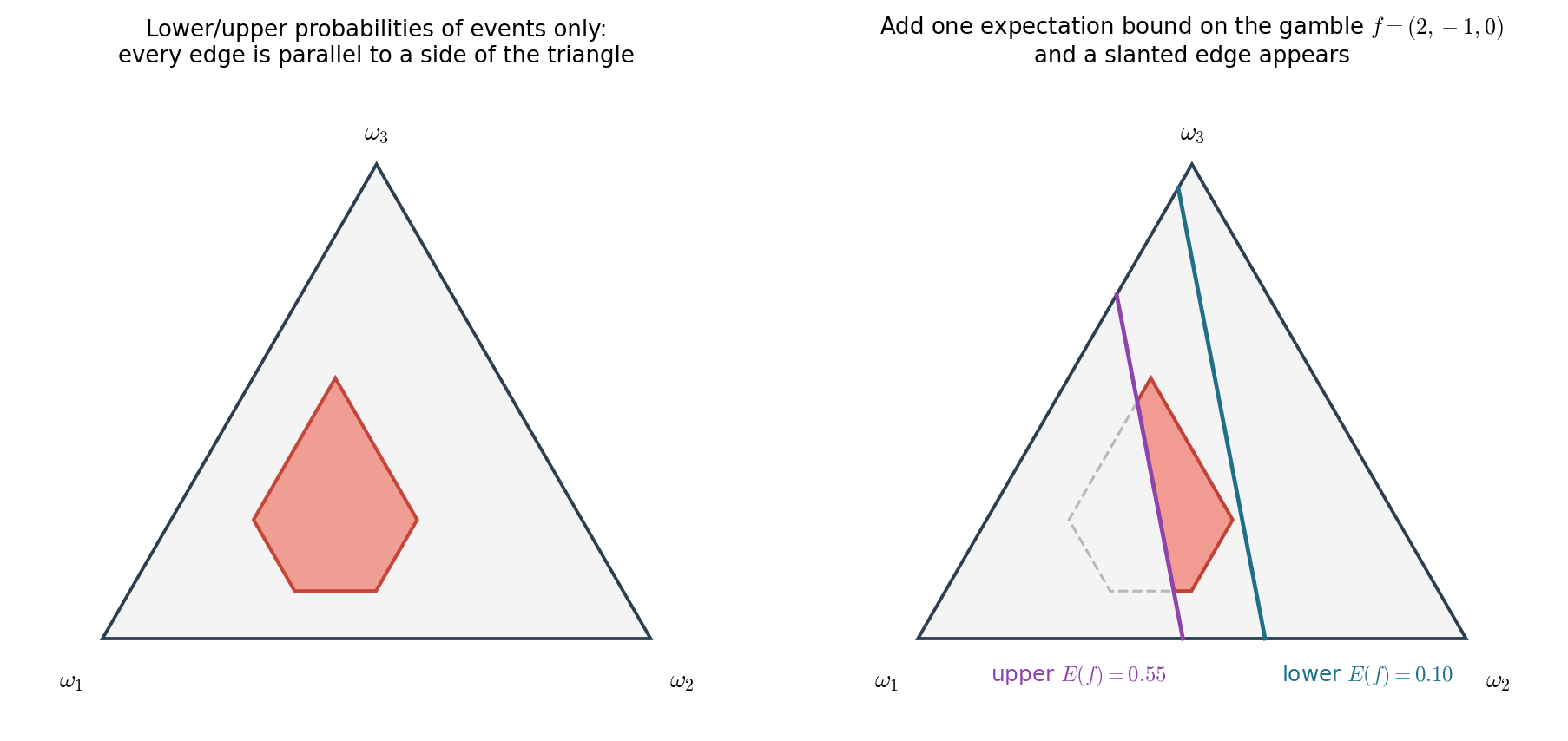
The left panel shows what can be achieved using only lower and upper probabilities of events: every edge is parallel to one of the triangle's sides. The right panel adds an expectation constraint for the gamble $f=(2,-1,0)$ , producing a slanted edge; the dashed outline shows the previous shape. Incidentally, adding a constant to $f$ does not change the direction of the line—it merely translates both boundaries together. Multiplying $f$ by a positive constant also leaves the direction unchanged, provided the bounds are scaled as well. The direction of the cut is therefore determined only by the relative differences among the components of $f$ . The gambles $f=(2,-1,0)$ , $f=(4,-2,0)$ , and $f=(3,0,1)$ all produce the same direction. I find this point quite important: writing down another $f$ does not necessarily introduce a new direction.

With several lower and upper expectation constraints, we can construct much more flexible credal sets:

K=\left\{ p\in\Delta_2: \underline E(f^{(j)}) \leq p\cdot f^{(j)} \leq \overline E(f^{(j)}), \ j=1,\ldots,m \right\}.

Each gamble supplies at most two potential boundaries. Intersecting all these half-planes with the probability simplex produces a convex polygon.

Constraints on event probabilities are merely a special case. If $f=I_A$ , then

E_p[I_A]=P_p(A).

Moving from lower and upper probabilities to lower and upper expectations is therefore not a completely new construction. It is a generalization from linear constraints with only $0$ – $1$ coefficients to arbitrary linear constraints.

From the viewpoint of convex geometry, the conclusion is even more direct. A closed convex set can be represented as an intersection of supporting half-spaces. If the credal set is a polytope, a finite collection of linear expectation constraints is enough to describe it. Conversely, if the desired convex set is not a polytope—consider a circle, for example—no finite collection of gambles can describe it exactly. We would need infinitely many, one supporting hyperplane in every direction. This also reveals the upper limit of the language: it describes convex sets. No matter how many gambles we add, they cannot produce a nonconvex credal set.

This, in my view, is what should be explained first. The gambling interpretation comes at a second level and should not be used to frighten beginners at the outset.

Buying and selling interpretations of lower and upper expectations

At this point, imprecise probability theory usually returns to the buying and selling interpretation of a gamble.

Suppose $f$ is a lottery ticket. The lower expectation, or lower prevision, $\underline E(f)$ can be understood as the highest price you are willing to pay to receive $f$ :

\underline E(f) =\sup\{\mu:f-\mu\text{ is a gamble you are willing to accept}\}.

If you pay $\mu$ to buy $f$ , your eventual net payoff is

f-\mu.

The higher the price, the less favorable the gamble becomes. The lower expectation is the limiting price you are still willing to accept.

The upper expectation, or upper prevision, $\overline E(f)$ can be understood as the lowest price at which you are willing to sell $f$ :

\overline E(f) =\inf\{\mu:\mu-f\text{ is a gamble you are willing to accept}\}.

The two are related by conjugacy:

\overline E(f)=-\underline E(-f).

When the lower and upper expectations agree, they reduce to a single precise fair price. When they leave an interval between them, the gap can be compared to a bid–ask spread.

My own way of understanding this, after setting the lottery language aside, is much simpler. We have a function $f$ whose payoff depends on the outcome, and we need to determine a plausible range for its expectation, by whatever method is available. If we want the most informative range, it should be as tight as possible. This naturally leads us to the greatest valid lower bound and the smallest valid upper bound.

I still do not find the buying-and-selling story especially intuitive. For me, it is much easier to begin with linear constraints, half-planes, and convex sets, and only then add that these bounds may also be interpreted as buying and selling prices. The interpretation is not useless, however. At least it supplies a consistency criterion: the lower and upper prices we quote must not combine to produce a guaranteed loss or a risk-free arbitrage. The notion of coherence is largely concerned with ruling out such internal contradictions.

Moreover, once a credal set $K$ has been specified, the two quantities have a particularly clean geometric meaning:

\underline E(f)=\min_{p\in K}p\cdot f, \qquad \overline E(f)=\max_{p\in K}p\cdot f.

We are simply optimizing a linear functional in the direction $f$ over $K$ . Since this is a linear program, an optimum occurs at a vertex of $K$ . If we have a list of those vertices, finding the lower and upper expectation of any gamble is just a matter of evaluating it at every vertex and taking the minimum and maximum. I find this far more useful than the language of buying and selling prices. It shows that lower and upper expectations and credal sets are two descriptions of the same object: one in terms of support values, the other in terms of the set itself.

Where do these constraints come from?

One might object that there are infinitely many gambles. Are we supposed to ask an expert for lower and upper prices for every one of them?

Of course not.

In a concrete problem, we should choose only gambles or statistics that genuinely matter to the task. Examples include:

the payoff of a particular decision in each state;
a loss function;
a plausible range for the expectation of a feature or indicator;
a small number of scenarios that an expert can understand and assess.

From these finitely many policies, payoff functions, or moment constraints, we can construct a credal set.

In this sense, the framework is indeed a way to model expert knowledge. Rather than asking an expert to draw a polygon directly inside the probability triangle, we ask: “For this particular payoff function, what range of expected values do you consider reasonable?” Several answers then cut out a set of plausible probability distributions.

There is also a conservative shortcut built into the framework. The fewer constraints we provide, the larger and more “ignorant” the resulting set will be—but at least it will not pretend that we know more than we do. In the theory, this is called natural extension: begin with the few commitments we are genuinely prepared to make, then take all probability distributions compatible with them. The result is the most conservative credal set consistent with those commitments. Asking about one more gamble makes the set smaller, or at least never larger. Asking nothing leaves us with the vacuous model. The virtue of this approach is that it does not force us to claim knowledge we do not possess; the drawback is that it can easily leave us unable to say anything useful.

If the constraints come mainly from subjective expert judgments, the final model will depend heavily on which gambles we choose to ask about, how we phrase the questions, and whether the expert can answer consistently. Anyone with a machine-learning background may find this a little dubious—I do too. It can feel suspiciously like hand-designing constraints all over again.

At least I can now reduce the idea to something concrete:

Use a collection of task-relevant linear expectation constraints to cut a convex set of plausible probability distributions out of the probability simplex.

Whether those constraints are reliable, reproducible, or worth eliciting is a separate question about modeling and knowledge acquisition. Another way to view the issue is that no nonlinear feature has appeared anywhere yet: everything consists of straight-line cuts. Linearity provides clean geometry and tractable computation. Nonlinear extensions can wait for a future discussion.

Summary

This note is really trying to make only a few points.

First, the ternary probability simplex is a triangle because the plane

p_1+p_2+p_3=1

is cut by the constraints

p_1,p_2,p_3\geq0.

Coordinates inside the triangle are normalized perpendicular distances to the opposite edges, and the three distances always sum to $1$ .

Second, a linear-vacuous credal set remains a triangle because it is an affine scaling of the full probability simplex:

K_\varepsilon=(1-\varepsilon)p^0+\varepsilon\Delta_2.

More intuitively, it is a homothety centered at $p^0$ with scale factor $\varepsilon$ . Other models—pari-mutuel, total-variation, COR, and probability-interval models—produce various triangles and hexagons. They are all convex polygons because all their constraints are linear inequalities.

Third, ordinary lower and upper probability constraints are special expectation constraints whose coefficients are only $0$ or $1$ , so the available cutting directions are limited. General lower and upper expectation constraints,

\underline E(f)\leq p\cdot f\leq\overline E(f),

can produce linear boundaries in any direction and hence much more flexible convex credal sets. Conversely, once $K$ is given, lower and upper expectations are obtained by minimizing and maximizing a linear functional over $K$ . They are two ways to describe the same object.

Fourth, gambling and buying or selling prices provide a behavioral interpretation, but they are not the only route to understanding the geometry. For me, vectors, planes, and convex sets make a much better starting point; gambles become easier to understand afterward.

The subject is not as mysterious as it initially appeared in the course. At bottom, it is convex geometry on a probability simplex, wrapped in the language of gambling so that it can be used for decision making. The more general a theory becomes, the more broadly it applies—and often the harder it becomes to put into practice. I will continue working through the later material gradually. The tentative title of the next post is Decision Philosophy and Choice Functions.